Calibrating Volatility Surfaces with Deep-Learning

1. Introduction
   1. Overview
   2. Dataset
2. Neural-Net Method
   1. Approach
   2. Architecture
   3. Training
   4. Performance – Testing Dataset
3. Heston Model
   1. Approach
   2. Performance – Testing Dataset
   3. Calibration – Interpretation Example
4. Comparative Results
5. Conclusion
6. References

Introduction

Overview

This use-case aims to compare the performance of two interpolation approaches for equity volatility surfaces: 1) Neural Net based method vs. 2) Heston stochastic volatility model.

The input dataset contains :

• 5 years of Nikkei daily volatility surfaces across 2015-2019
• Black-Scholes volatilities inferred from historical data of option prices

Dataset

The raw dataset is provided along with the academic paper listed in References [1].

Each observation σ_i is located on the grid through its coordinates (T_i,Moneyness_i) where:

• σ_i: Black-Scholes Log Normal volatility
• T_i: Maturity expressed in years
• Moneyness_i: high moneyness here refers to lower strikes

Summary:

• Number of reference days in the dataset: 1296
• Maximum number of maturities per reference date: 15
• Maximum number of moneyness points per maturity: 17
• The grid coordinates are dynamic across the reference dates

Neural-Net Method

Approach

The neural net is trained to reconstruct the volatility surfaces over the training dataset. The dataset is divided into a training dataset and a testing dataset. The training dataset represents 80% of the chronologically ordered observations, i.e. 4 years of data spanning 2015-2018 (31 December 2018 excluded). The underlying assumption is the lower the reconstruction error, the more accurate the interpolator would be on points not in the volatility grid.

The so-called neural net is comprised of two neural nets: an encoder and a decoder:

Encoder: theoretically, any injective map from a relevant subset S of R^m to a space R^f of factors where f<<m. The encoder serves as a compressor by reducing the dimensionality of the input, much like a principal component analysis. Unlike the PCA, however, the encoder is a non-linear function

Decoder: conversely, the decoder reconstructs the values of an input tensor from any set of factors; D : R^f -> S

Architecture

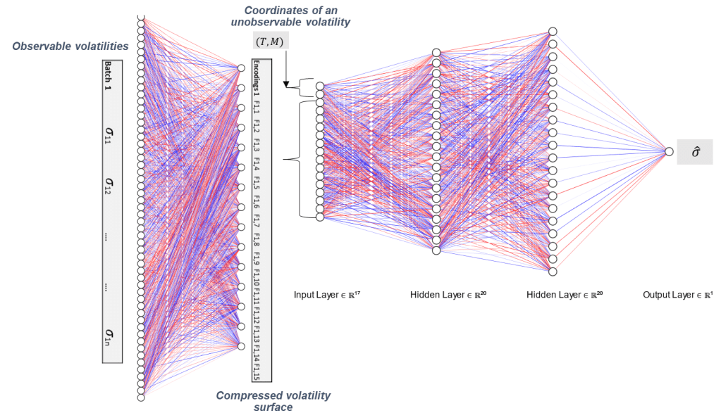
• The encoder is a dense layer with 15 factors or output units
• 15 factors are commonly used in PCAs by equity derivatives trading. See References [1]
• The PCA shows that 9 factors explain 99% of variance of volatilities in the dataset
• The decoder is a feed-forward neural network composed of three fully-connected layers with 20, 20 and 1 units

Training

1. For each iteration (i.e. epoch), a random sub-set of the training dataset is selected. A given batch of observable volatilities flows through the encoder
2. For each observable volatility, the input tensor is (Maturity, Moneyness, 15 factors). The encodings are replicated for all the individual volatilities “CodeTensor=Code.repeat(n,1)”
3. The decoder estimates one volatility at a time
4. Errors in each batch are aggregated into a mean square error for the whole sub-set
5. The decoder loss gradient with regard to the decoder weights are computed. The weights are updated accordingly
6. The encoder loss is copied on the decoder loss value. The gradient with regard to the encoder weights are computed. The (encoder) weights are updated accordingly

The training of the encoder solves for the minimum reconstruction error of the decoder. The training occurs once a year, based on the 4 past years of daily volatility surfaces. Other configurations could be explored. The interpolation of unobserved volatilities within future daily surfaces (i.e. out of sample) implies the determination of the factors/encodings of the new surface. To do so:

1. The encoder is “retrained” to minimize the reconstruction error of the decoder
2. The decoder is kept unchanged form the overall training; the trained decoder weights are kept constant
3. The factors all with the coordinates of the unobserved volatility are processed by the trained encoder

Note that non-arbitrage hypothesis is not tested here on interpolated volatilities.

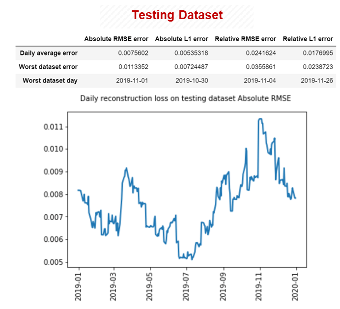
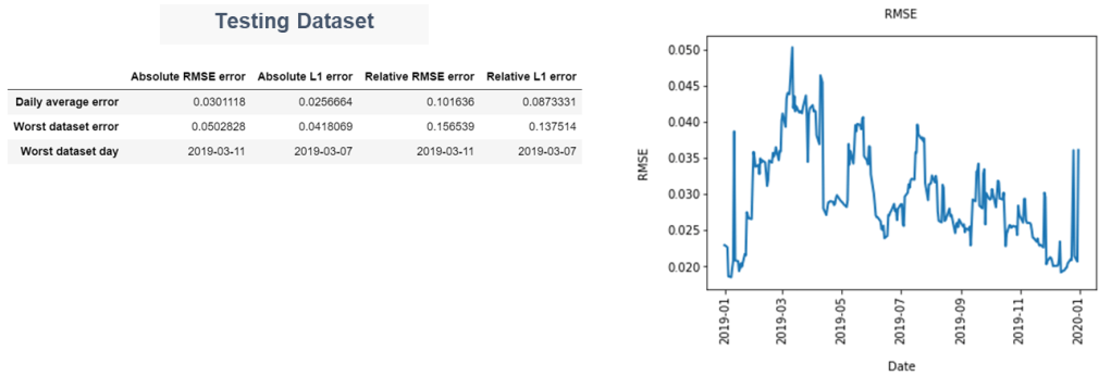
Performance – Testing Dataset

RMSE and L1 refer to mean square error and 1^st order error, respectively. Errors show no overfitting in the model. Overall, errors remain low (RMSE, L1 <1%). References[1] shows lower errors with more computing power.

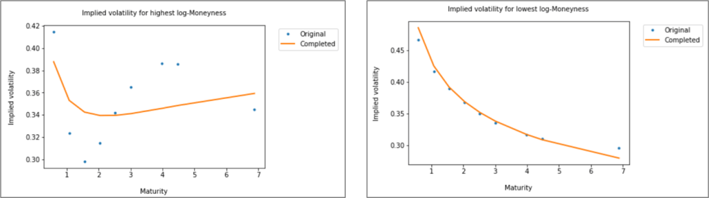
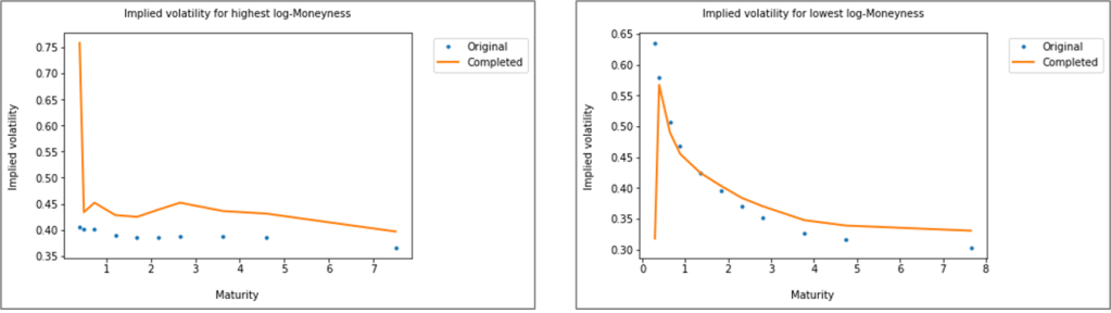
The charts below highlight the estimated vs. actual values of volatilities with highest (respectively lowest) moneyness, for the reference day with highest RMSE in the testing dataset (i.e. 01 November 2019). While the method reconstructs accurately the higher strikes, it does not capture well the lower ones regardless of the maturity. Lower strikes volatility curve below is also significantly distorted. The reconstructed surface is inline with the absence of arbitrage condition as commonly defined for calendar spreads.

Heston Model

Approach

Heston model is calibrated for each reference date over the testing dataset. For each maturity in the daily surface, the calibration is performed separately. The assumption is the lower the reconstruction error, the more accurate the interpolator would be on points not in the volatility grid.

Quantlib library is used to calibrate the model. Moreover, the risk-free interest rate curve is assumed flat and constant over time.

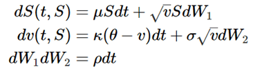
As a reminder, the asset in Heston is modeled as a stochastic process that depends on volatility v. The latter is a mean reverting stochastic process with a constant volatility of volatility σ. The two processes have a correlation ρ:

Performance – Testing Dataset

Overall, errors remain moderate. RMSE and L1 errors are higher when compared to the neural net approach by a fold of approximately 4x over the same period.

The charts below highlight the estimated vs. actual values of volatilities with highest (respectively lowest) moneyness for the reference day with highest RMSE in the testing dataset, i.e. 11 March 2019. Except for the short maturities, the model reconstructs more accurately the higher strikes than the lower ones. Short maturities options have small Vega (and theta) exposures, thus the impact of such errors on P&L is immaterial. The reconstructed surface is inline with the absence of arbitrage condition as commonly defined for calendar spreads.

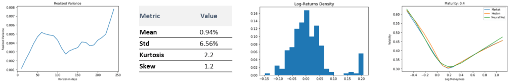
Calibration – Interpretation Example

Looking at realized 5m returns over [2015-2018] highlights a kurtosis, i.e. fat tailed distribution which justifies the smile (non-gaussian density). The smile is skewed toward higher returns given the skew metric above 1. We expected higher strikes implied volatilities (or OTM calls implied volatilities) to be higher than lower strikes ones. A positive spot shock is more likely to be accompanied by a positive volatility shock.

The right chart shows the 5m volatility smile at 31 Dec 2018 reference date, we can infer that rho is positive. The realized Variance shows varying slopes and different signs. The initialization of θ and κ parameters can also be challenging.

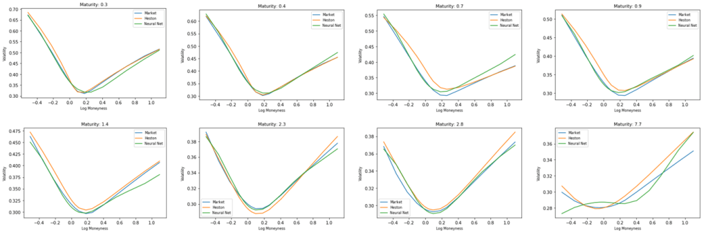
Comparative Results

Reconstructed curves : Reference Date 31 December 2018

The charts below highlight the actual volatilities vs. estimated values according to the two approaches, per maturity. Overall, the neural net approach is more accurate than Heston model except for the highest maturity curve. Accuracy around ATM could be improved (in theory) by adding more observable points around it and/or masking few lower strikes volatilities in the training dataset.

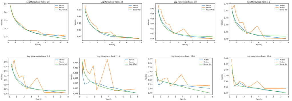
The charts below highlight the actual volatilities vs. estimated values according to the two approaches, per moneyness. Since the grid is dynamic, we grouped volatilities according to their respective ranks, i.e. Rank(Moneyness_i). Unlike Heston Model, the neural net interpolation is more consistent across (K,T).

Conclusion

Neural Net: accuracy is high overall and is consistent across strikes and maturities. The accuracy is cross-checked with linear interpolation whose performance remains comparable. The biggest weakness is in the very long-term volatilities (>7years in this study). Though computing power could be a hurdle, the training is performed only once a year.

Heston: the biggest weakness lies in the difficulty of the calibration. Other weaknesses include inconsistencies in calibrated volatilities across the same moneyness. The main advantages are good accuracy when combined with a market expertise, especially on the long-term maturities.

Some of the conclusions were generalized from specific cases without thorough statistical checks.

References

1. Neural Net based method : “Nowcasting Networks – Marc Chataigner, Stephane Crépey, and Jiang Pu” [2020]
2. Heston model: https://www.quantlib.org/docs.shtml